前言
之前介绍了FGSM算法还有I-FGSM算法,接下来再看看FGSM算法的拓展PGD算法。
PGD原理
PGD算法在论文[1706.06083] Towards Deep Learning Models Resistant to Adversarial Attacks (arxiv.org)中提出,它既是产生对抗样本的攻击算法,也是对抗训练的防御算法。除此之外,PGD算法也是一阶中的最强攻击(一阶是指利用一阶导数)
设想目标模型如果是一个线性模型,损失函数对输入的导数一定是一个固定值,一次迭代和多次迭代时扰动的方向都不会发生改变,但是,如果目标模型为非线性,每次迭代之间的方向都有可能会发生变化,这时FGSM的单次迭代效果肯定不如PGD的效果好。FGSM算法通过一步计算,可能达不到最优效果,而PGD算法则是每次走一小步,但是多走几次,如果超过了扰动半径为ε的空间,就重新映射回来。
下面来看一下PGD算法的公式:
就是通过一系列操作得到对抗样本后,将对抗样本减去原始图像得到了扰动值,然后将扰动值限制在-ε到+ε之间,得到了新的扰动值,原始图像加上新的扰动值就是最终生成的对抗样本。
关于我对(1)中sgn(L(θ,x,y)’)的理解可以看我在这篇文章中2.1节写的内容。对抗攻击:FGSM和BIM算法 | WeiSJ&HEXO (lengnian.github.io)
Pytorch代码实现
看看PGD的核心代码:
# PGD攻击方式,属于FGSM攻击的变体
def PGD_attack(model, image, label, epsilon=0.8, alpha=0.1, iters=40):
    image = image.to(device)
    label = label.to(device)
    loss = nn.CrossEntropyLoss()

    ori_image = image.data

    for i in range(iters):
        image.requires_grad = True
        output = model(image)

        model.zero_grad()
        cost = loss(output, label).to(device)
        cost.backward()

        # 对抗样本 = 原始图像 + 扰动
        adv_image = image + alpha * image.grad.sign()
        # 限制扰动范围
        eta = torch.clamp(adv_image - ori_image, min=-epsilon, max=epsilon)
        # 进行下一轮的对抗样本生成
        image = torch.clamp(ori_image + eta, min=0, max=1).detach()

    return image
训练+攻击完整代码
完整代码是使用自己在MNIST手写数据集上训练的LeNet,使用PGD算法产生对抗样本攻击模型。
首先是模型搭建
# 搭建LeNet模型
class LeNet(nn.Module):
    def __init__(self):
        super(LeNet, self).__init__()

        # 卷积层
        self.conv = nn.Sequential(
            nn.Conv2d(in_channels=1, out_channels=6, kernel_size=5, padding=2),
            nn.ReLU(),
            nn.MaxPool2d(kernel_size=2, stride=2),
            nn.Conv2d(in_channels=6, out_channels=16, kernel_size=5),
            nn.ReLU(),
            nn.MaxPool2d(kernel_size=2, stride=2)
        )

        # 全连接层
        self.fc = nn.Sequential(
            nn.Linear(in_features=16 * 5 * 5, out_features=120),
            nn.ReLU(),
            nn.Linear(in_features=120, out_features=84),
            nn.ReLU(),
            nn.Linear(in_features=84, out_features=10)
        )

    def forward(self, img):
        img = self.conv(img)
        img = img.view(img.size(0), -1)
        out = self.fc(img)
        return out


net = LeNet()
net = net.to(device)
mean = 0.1307
std = 0.3801
# 对图像变换
transform = transforms.Compose([
transforms.ToTensor(),
transforms.Normalize((mean,), (std,))
]
)
device = torch.device("cuda" if torch.cuda.is_available() else "cpu")# 训练数据集, 测试数据集
train_dataset = datasets.MNIST('../datasets/MNIST', train=True, transform=transform, download=True) # len 60000
test_dataset = datasets.MNIST('../datasets/MNIST', train=False, transform=transform, download=True) # len 10000
# 数据迭代器
train_dataloader = DataLoader(train_dataset, batch_size=64, shuffle=True) # len 938
test_dataloader = DataLoader(test_dataset, batch_size=64, shuffle=True) # len 157
lr = 1e-3
epochs = 30
optimizer = torch.optim.Adam(net.parameters(), lr=lr)
criterion = nn.CrossEntropyLoss()
scheduler = torch.optim.lr_scheduler.ReduceLROnPlateau(optimizer, 'min', factor=0.5, verbose=True, patience=5, min_lr=0.0000001)之后就是进行模型的训练
train_loss = []
train_acc = []
val_loss = []
val_acc = []
for epoch in tqdm(range(epochs)):
train_losses = 0
train_acces = 0
val_losses = 0
val_acces = 0
for x, y in train_dataloader:
x, y = x.to(device), y.to(device)
output = net(x)
# 计算loss
loss = criterion(output, y)
# 计算预测值
_, pred = torch.max(output, axis=1)
# 计算acc
acc = torch.sum(y == pred) / output.shape[0]
# 反向传播
# 梯度清零
optimizer.zero_grad()
loss.backward()
optimizer.step()
train_losses += loss.item()
train_acces += acc.item()
train_loss.append(train_losses / len(train_dataloader))
train_acc.append(train_acces / len(train_dataloader))
# 模型评估
net.eval()
with torch.no_grad():
for x, y in test_dataloader:
x, y = x.to(device), y.to(device)
output = net(x)
loss = criterion(output, y)
scheduler.step(loss)
_, pred = torch.max(output, axis=1)
acc = torch.sum(y == pred) / output.shape[0]
val_losses += loss.item()
val_acces += acc.item()
val_loss.append(val_losses / len(test_dataloader))
val_acc.append(val_acces / len(test_dataloader))
print(f"epoch:{epoch+1} train_loss:{train_losses / len(train_dataloader)}, train_acc:{train_acces / len(train_dataloader)}, val_loss:{val_losses / len(test_dataloader)}, val_acc:{val_acces / len(test_dataloader)}")
plt.plot(train_loss, color='green', label='train loss')
plt.plot(val_loss, color='blue', label='val loss')
plt.legend()
plt.xlabel("epoch")
plt.ylabel("loss")
plt.show()
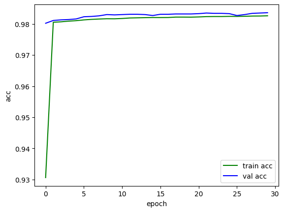
plt.plot(train_acc, color='green', label='train acc')
plt.plot(val_acc, color='blue', label='val acc')
plt.legend()
plt.xlabel("epoch")
plt.ylabel("acc")
plt.show()
PATH = './pgd_mnist_lenet.pth'
torch.save(net, PATH) 3%|▎ | 1/30 [00:11<05:30, 11.39s/it]
epoch:1 train_loss:0.22698007381932217, train_acc:0.9306369936034116, val_loss:0.06039735894490057, val_acc:0.9801950636942676
7%|▋ | 2/30 [00:21<05:05, 10.90s/it]
epoch:2 train_loss:0.06332400290375904, train_acc:0.980527052238806, val_loss:0.059576493097694624, val_acc:0.9810907643312102
10%|█ | 3/30 [00:32<04:48, 10.70s/it]
epoch:3 train_loss:0.06275213833576612, train_acc:0.9806603144989339, val_loss:0.05885813971328887, val_acc:0.9812898089171974
13%|█▎ | 4/30 [00:42<04:27, 10.28s/it]
epoch:4 train_loss:0.0622245114612411, train_acc:0.9808768656716418, val_loss:0.05824386749778441, val_acc:0.9813893312101911
17%|█▋ | 5/30 [00:52<04:18, 10.34s/it]
epoch:5 train_loss:0.06163326848739151, train_acc:0.9810267857142857, val_loss:0.05831151023495254, val_acc:0.9815883757961783
20%|██ | 6/30 [01:03<04:10, 10.45s/it]
epoch:6 train_loss:0.06115677414128362, train_acc:0.9812766524520256, val_loss:0.05730052098222552, val_acc:0.9822850318471338
23%|██▎ | 7/30 [01:14<04:06, 10.71s/it]
epoch:7 train_loss:0.06073849064423077, train_acc:0.9814432302771855, val_loss:0.0568622479387292, val_acc:0.9823845541401274
27%|██▋ | 8/30 [01:24<03:52, 10.57s/it]
epoch:8 train_loss:0.060348112858943086, train_acc:0.9815598347547975, val_loss:0.05643120593136283, val_acc:0.9825835987261147
30%|███ | 9/30 [01:36<03:53, 11.12s/it]
epoch:9 train_loss:0.06001822312654399, train_acc:0.9816431236673774, val_loss:0.0560989200529067, val_acc:0.9829816878980892
33%|███▎ | 10/30 [01:47<03:40, 11.01s/it]
epoch:10 train_loss:0.05972875392924287, train_acc:0.9816264658848614, val_loss:0.055768566766670746, val_acc:0.9828821656050956
37%|███▋ | 11/30 [02:00<03:37, 11.44s/it]
epoch:11 train_loss:0.05945397531891714, train_acc:0.9817264125799574, val_loss:0.05558454929880655, val_acc:0.9829816878980892
40%|████ | 12/30 [02:10<03:21, 11.21s/it]
epoch:12 train_loss:0.05924657509594695, train_acc:0.9818929904051172, val_loss:0.05523945889465368, val_acc:0.9830812101910829
43%|████▎ | 13/30 [02:24<03:22, 11.89s/it]
epoch:13 train_loss:0.05902852281344248, train_acc:0.9819429637526652, val_loss:0.05497432513508032, val_acc:0.9830812101910829
47%|████▋ | 14/30 [02:39<03:25, 12.82s/it]
epoch:14 train_loss:0.05884089107651994, train_acc:0.9819929371002132, val_loss:0.05479716256581199, val_acc:0.9829816878980892
50%|█████ | 15/30 [02:51<03:09, 12.62s/it]
epoch:15 train_loss:0.05864403824453979, train_acc:0.9820429104477612, val_loss:0.05505548159378302, val_acc:0.9826831210191083
53%|█████▎ | 16/30 [03:03<02:54, 12.50s/it]
epoch:16 train_loss:0.05848915197192502, train_acc:0.9820262526652452, val_loss:0.05448126511731345, val_acc:0.9830812101910829
57%|█████▋ | 17/30 [03:14<02:35, 11.96s/it]
epoch:17 train_loss:0.05836289135941755, train_acc:0.9820429104477612, val_loss:0.05426665444437201, val_acc:0.9830812101910829
60%|██████ | 18/30 [03:26<02:25, 12.09s/it]
epoch:18 train_loss:0.05820710067130895, train_acc:0.9821761727078892, val_loss:0.054053511006377966, val_acc:0.9831807324840764
63%|██████▎ | 19/30 [03:38<02:12, 12.01s/it]
epoch:19 train_loss:0.058103710266032706, train_acc:0.9821761727078892, val_loss:0.05439911206745228, val_acc:0.9831807324840764
67%|██████▋ | 20/30 [03:49<01:56, 11.64s/it]
epoch:20 train_loss:0.058076391998888935, train_acc:0.9821595149253731, val_loss:0.05379035640181677, val_acc:0.9831807324840764
70%|███████ | 21/30 [04:01<01:46, 11.86s/it]
epoch:21 train_loss:0.0578732310768479, train_acc:0.9822261460554371, val_loss:0.05364397724283634, val_acc:0.98328025477707
73%|███████▎ | 22/30 [04:12<01:32, 11.57s/it]
epoch:22 train_loss:0.05777005526695901, train_acc:0.9823260927505331, val_loss:0.05357255679510747, val_acc:0.9834792993630573
77%|███████▋ | 23/30 [04:25<01:24, 12.03s/it]
epoch:23 train_loss:0.05769451945396597, train_acc:0.982359408315565, val_loss:0.05339814494749543, val_acc:0.9833797770700637
80%|████████ | 24/30 [04:38<01:14, 12.38s/it]
epoch:24 train_loss:0.05762437407273863, train_acc:0.982359408315565, val_loss:0.05328276433023939, val_acc:0.9833797770700637
83%|████████▎ | 25/30 [04:52<01:03, 12.70s/it]
epoch:25 train_loss:0.057558819814188, train_acc:0.982409381663113, val_loss:0.0532996576148898, val_acc:0.98328025477707
87%|████████▋ | 26/30 [05:04<00:50, 12.55s/it]
epoch:26 train_loss:0.05746660577848172, train_acc:0.9823927238805971, val_loss:0.05423711911051469, val_acc:0.9826831210191083
90%|█████████ | 27/30 [05:15<00:35, 11.98s/it]
epoch:27 train_loss:0.05736568021470868, train_acc:0.982442697228145, val_loss:0.053538712084139135, val_acc:0.9829816878980892
93%|█████████▎| 28/30 [05:25<00:23, 11.61s/it]
epoch:28 train_loss:0.057331098256998066, train_acc:0.9825093283582089, val_loss:0.053118417597120736, val_acc:0.9833797770700637
97%|█████████▋| 29/30 [05:36<00:11, 11.26s/it]
epoch:29 train_loss:0.05727743341136716, train_acc:0.982525986140725, val_loss:0.05280723534694985, val_acc:0.9834792993630573
100%|██████████| 30/30 [05:48<00:00, 11.62s/it]
epoch:30 train_loss:0.05723029628682977, train_acc:0.982592617270789, val_loss:0.05286279270294935, val_acc:0.9835788216560509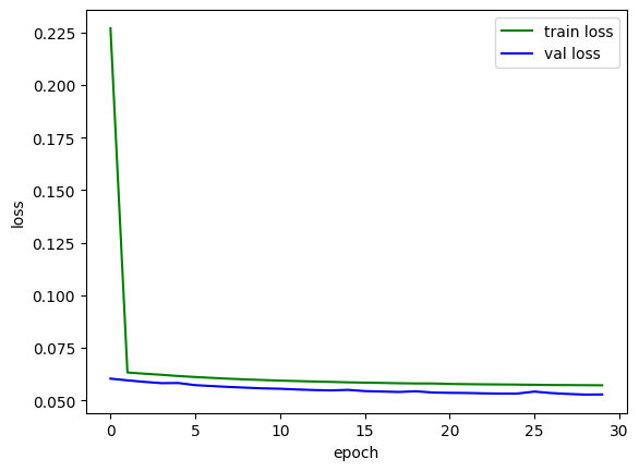
为了方便后续的可视化,将测试数据集加载器的bathsize设置为1。
test_dataloader = DataLoader(test_dataset, batch_size=1, shuffle=True) PGD算法
# PGD攻击方式,属于FGSM攻击的变体
def PGD_attack(model, image, label, epsilon=0.8, alpha=0.1, iters=40):
    image = image.to(device)
    label = label.to(device)
    loss = nn.CrossEntropyLoss()

    ori_image = image.data

    for i in range(iters):
        image.requires_grad = True
        output = model(image)

        model.zero_grad()
        cost = loss(output, label).to(device)
        cost.backward()

        # 对抗样本 = 原始图像 + 扰动
        adv_image = image + alpha * image.grad.sign()
        # 限制扰动范围
        eta = torch.clamp(adv_image - ori_image, min=-epsilon, max=epsilon)
        # 进行下一轮的对抗样本生成
        image = torch.clamp(ori_image + eta, min=0, max=1).detach()

    return image
测试函数
def test_PGD(model, device, test_dataloader, epsilon, alpha):
    correct = 0
    adv_examples = []

    for data, target in test_dataloader:
        data, target = data.to(device), target.to(device)
        data.requires_grad = True

        output = model(data)
        _, init_pred = torch.max(output, axis=1)
        # print("origin label", init_pred)

        # 分类错误就不去扰动图像
        if init_pred.item() != target.item():
            continue

        # 使用PGD进行攻击
        perturbed_image = PGD_attack(model, data, target, epsilon=epsilon, alpha=alpha)
        output = model(perturbed_image)
        _, attack_pred = torch.max(output, axis=1)
        # print("attack label", attack_pred)

        # 扰动后还是分类正确
        if attack_pred.item() == target.item():
            correct += 1
        else:
            # print("classifier failed!")
            if len(adv_examples) < 5:
                adv_ex = perturbed_image.squeeze().detach().cpu().numpy()
                adv_examples.append((init_pred.item(), attack_pred.item(), adv_ex))

    attack_acc = correct / len(test_dataloader)
    print("    Epsilon: {}\tTest Accuracy = {} / {} = {}".format(epsilon, correct, len(test_dataloader), attack_acc))

    return adv_examples, attack_acc
使用PGD算法生成对抗样本并计算准确率,在这里我使ε和α都发生变化
accuracies = []
examples = []
epsilons = [0.4, 0.5, 0.6]
alphas = [2/255, 2/128, 2/64, 2/32]

for alpha in alphas:
    print("Alpha:{:.5f}".format(alpha))
    for epsilon in epsilons:
        ex, acc = test_PGD(net, device, test_dataloader, epsilon=epsilon, alpha=alpha)
        accuracies.append(acc)
        examples.append(ex)
# 测试结果
Alpha:0.00784
Epsilon: 0.4 Test Accuracy = 8453 / 10000 = 0.8453
Epsilon: 0.5 Test Accuracy = 4201 / 10000 = 0.4201
Epsilon: 0.6 Test Accuracy = 1075 / 10000 = 0.1075
Alpha:0.01562
Epsilon: 0.4 Test Accuracy = 8113 / 10000 = 0.8113
Epsilon: 0.5 Test Accuracy = 3093 / 10000 = 0.3093
Epsilon: 0.6 Test Accuracy = 488 / 10000 = 0.0488
Alpha:0.03125
Epsilon: 0.4 Test Accuracy = 8160 / 10000 = 0.816
Epsilon: 0.5 Test Accuracy = 2991 / 10000 = 0.2991
Epsilon: 0.6 Test Accuracy = 402 / 10000 = 0.0402
Alpha:0.06250
Epsilon: 0.4 Test Accuracy = 8265 / 10000 = 0.8265
Epsilon: 0.5 Test Accuracy = 3098 / 10000 = 0.3098
Epsilon: 0.6 Test Accuracy = 406 / 10000 = 0.0406可视化测试结果
alpha_1 = accuracies[:3]
alpha_2 = accuracies[3:6]
alpha_3 = accuracies[6:9]
alpha_4 = accuracies[9:]


plt.figure(figsize=(20,15))
plt.plot(epsilons, alpha_1, "b*-", label='Alpha=0.0078')
plt.plot(epsilons, alpha_2, "r*-", label="Alpha=0.0126")
plt.plot(epsilons, alpha_3, "g*-", label="Alpha=0.0312")
plt.plot(epsilons, alpha_4, "*-", label="Alpha=0.0625")

plt.legend()
plt.title("Accuracy vs Epsilon and Alpha")
plt.xlabel("Epsilon")
plt.ylabel("Accuracy")
plt.show()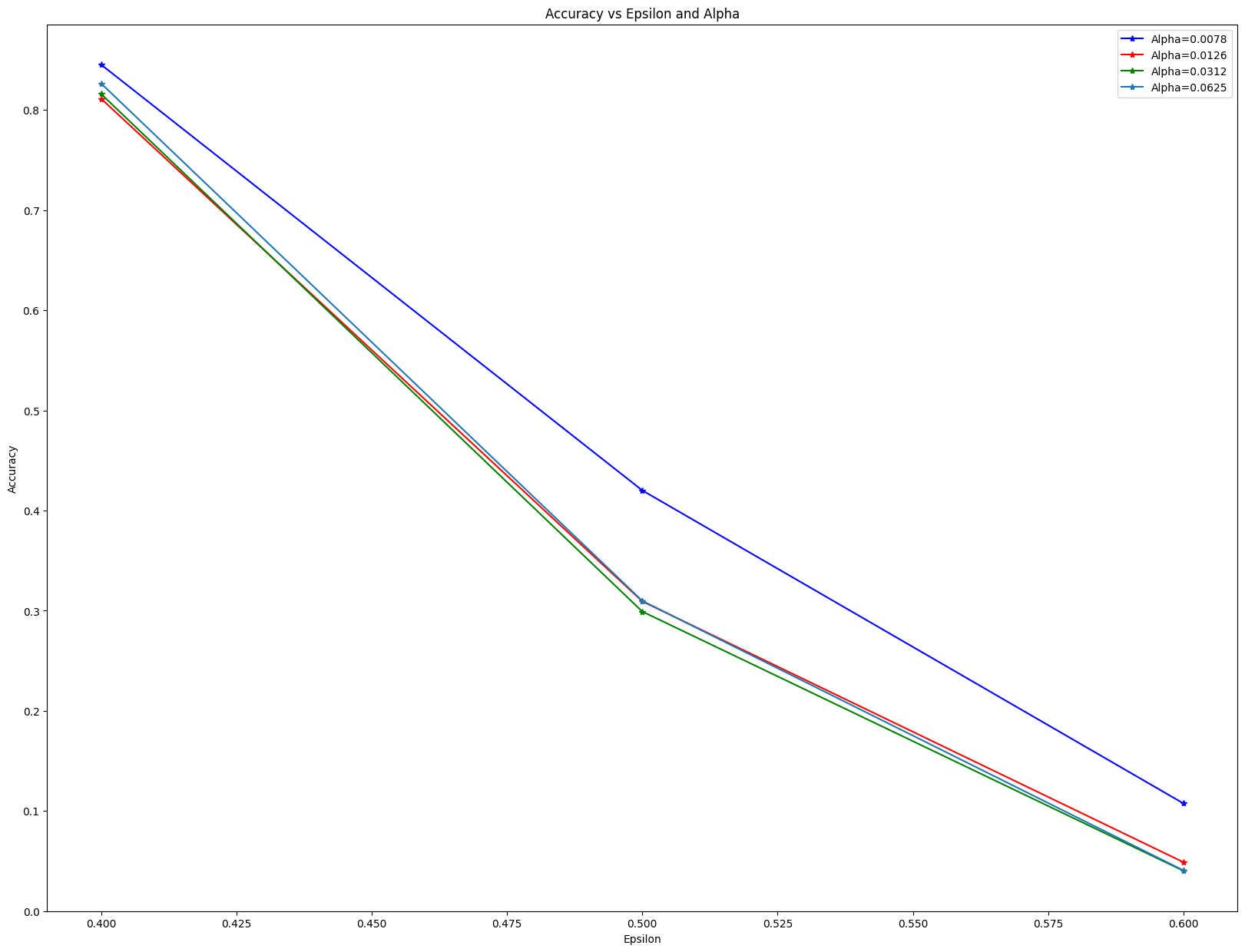
可视化不同参数下的对抗样本
index = 0
plt.figure(figsize=(15, 20))

for i in range(len(examples)):
    for j in range(len(examples[i])):
        index += 1
        plt.subplot(len(examples), len(examples[i]), index)
        if j == 0:
            if index <= 15:
                plt.ylabel("Eps:{} Alpha:{}".format(epsilons[i%3], 0.0078), fontsize=10)
            elif index > 15 and index <= 30:
                plt.ylabel("Eps:{} Alpha:{}".format(epsilons[i%3], 0.0126), fontsize=10)
            elif index > 30 and index <= 45:
                plt.ylabel("Eps:{} Alpha:{}".format(epsilons[i%3], 0.0312), fontsize=10)
            else:
                plt.ylabel("Eps:{} Alpha:{}".format(epsilons[i%3], 0.0625), fontsize=10)

        init_pred, attack_pred, example = examples[i][j]
        plt.title("{} --> {}".format(init_pred, attack_pred))
        plt.imshow(example)

plt.tight_layout()
# plt.show()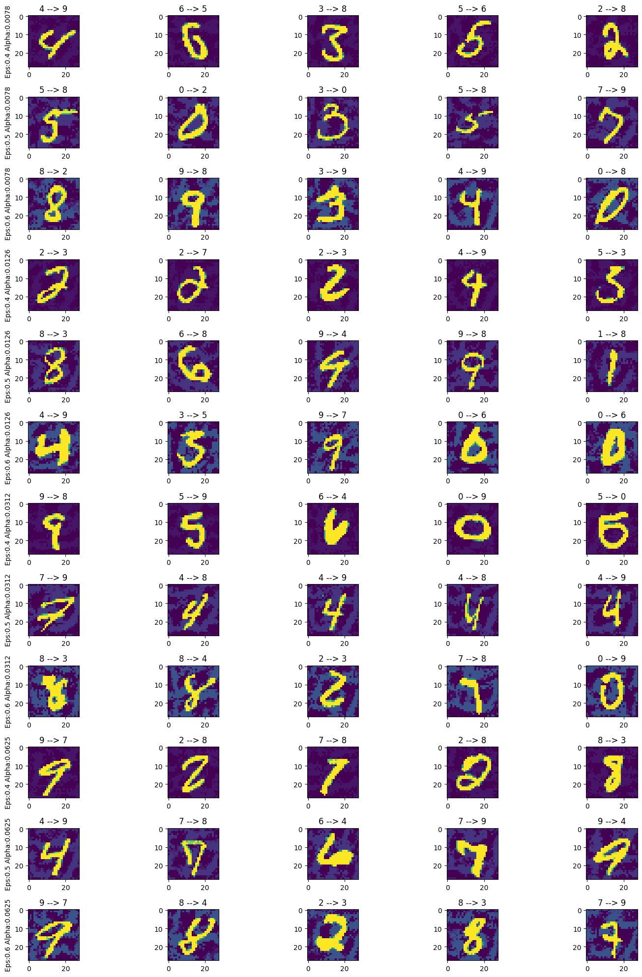
参考文献
对抗训练fgm、fgsm和pgd原理和源码分析-CSDN博客
3.基于梯度的攻击——PGD - 机器学习安全小白 - 博客园 (cnblogs.com)
对抗攻击篇:FGSM 与 PGD 攻击算法 | Just for Life. (muyuuuu.github.io)(能力有限,核心代码参考该作者)
